Welcome to the blog for my Creative Practice Music Project at the University of Edinburgh. This blog outlines the six month development of this project between October 2018 and April 2019. For an explanation of the mechanics the Fourier Transform and the code used, refer to the writeup that accompanies the project download.
Between electing to take this on this project in mid-October and today, I have engaged in research for the project. James McCellen, Ronald Schafer and Mark Yoder’s book Signal Processing First proved to be immensely insightful. Through reading this book and enrolling on the module ‘Musical Applications of Fourier Theory and Digital Signal Processing’, I have been able to learn about the intricacies of the of the Discrete Short Time Fourier Transform (DSTFT) before thinking about how it will be applied in Max. I am glad that I have a fundamental understanding of the process, which I’m sure will prove useful further down the line.
Pieces of work that I would recommend to anyone interested in this topic:
Luke Dubois‘ ‘jitter_pvoc_2D’, which is located in the example directory in Max 8 (/Users/jack/Library/Application Support/Cycling ’74/Max 8/Examples/jitter-examples/audio/jitter_pvoc).
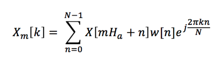
Over the past few weeks I have been investigating which equations will be relevant to the project I want to build. In the lecture notes for for MAFTDSP I came across the equation for DSTFT.
The equation for the DSTFT
While intimidating to look at at first, what this formula outlines is a process where a signal is broken down into a series of shorter horizontal segments called ‘frames’, where each frame is then analysed according to a certain number of vertical frequency ‘bin’s.
Between reading through James McCellan’s, Ronald Schafer’s and Mark Yoder’s Signal Processing First and the lecture notes for MAFTDSP I have been able to teach myself the mechanics of the Fourier Transform in the context of the DSTFT. One concept that took me a while to grasp was how the complex exponential in each frequency bin interaction with the input signal. Windowing (or framing), frequency bins, hop size, etc. are all relatively straightforward insofar as you can pinpoint where they are on a waveform and to me to they are tied to it in a logical way. What was the hardest for me to grasp was the link between not only how a real and imaginary number create a ‘spinning’ complex exponential on the complex plane, but also how this exponential would indicate frequency levels of an input signal in certain bins. Similarly with phase information, I found being able to picture how the relatively abstracted process of wrapping the phase information between -π and π would be useful in signal reconstruction in Max
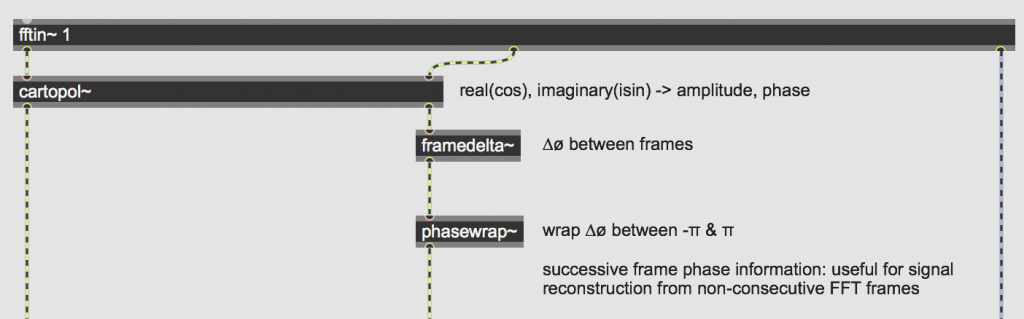
Perhaps somewhat ironically, or intuitively (depending on how you’re look at it), it was after studying Luke Dubois’ ‘jitter_pvoc_2D’ in Max’s example patches that I understood how these mathematical concepts were rendered in the Max environment.
The directory path where you can find Luke Dubois’ ‘jitter_pvoc_2D’: /Cycling ’74/Max 8/Examples/jitter-examples/audio/jitter_pvoc
The ‘cartopol~’ object in the above image is what solidified my understanding of how a complex number (complex in the mathematical sense of being composed of real and imaginary values) could be processed by a computer. The idea of a computer or any physical system being able to process an imaginary number is completely non-sensical, and it was upon discovering the ‘cartopol~’ object that the process made sense to me.
For ‘framedelta~’ and ‘phasewrap~’ to operate, they must receive signal in tangible polar coordinate form. The object ‘cartopol~’ is necessary because in its pure form, Fourier Analysis of a signal outputs data in Cartesian coordinates, i.e. as as a coordinate in relation to real (cosine) and imaginary (sin) axis on the complex plane.
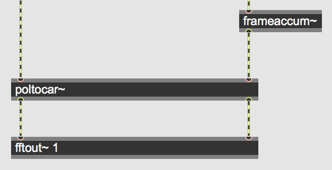
The concepts of running phase calculation, and frequency deviation were grounded in terms of my understandings in the ‘frameaccum~’ and ‘fftout~’ objects.
While Jean François-Charles’ article is completely seminal in terms of its explanation of spectral processing once the user has acquired their DSTFT data, he does not explain how to collect that data in Max in the first place. This had always been the most mystifying part of the process to me, so over the last few weeks I have been studying studying Luke Dubois’ jitter_pvoc_2D and Cycling 74’s article on implementing phase vocoders in Max.
The directory path where you can find Luke Dubois’ ‘jitter_pvoc_2D’: /Cycling ’74/Max 8/Examples/jitter-examples/audio/jitter_pvoc
I’m glad that Max has the functionality to be able to offer the user a relatively large freedom in terms of how they want to conduct the DSTFT, this choice has left me slightly overwhelmed. There have been two major choices to make in relation to DSTFT data collection: whether to use the ‘fft~’ or ‘fftin~’ object (inside a ‘pfft~’) and whether to use a ‘jit.matrix’ or a ‘buffer~’ to actually store the data. While the exact differences between the options are outlined in my project writeup in ‘1.1 main’, it is worth mentioning that both Jean François-Charles, Luke Dubois and Cycling 74 advised against the ‘fft~’ object, as it does not offer as much in-built functionality as ‘fftin~’.
One distinction I also struggled with was that between frame size and spectral frame size. Speaking to my supervisor and investigated the effect of the Nyquist frequency on DSTFT data collection really cleared this confusion up for me. As I have the full spectrum flag disabled on the ‘pfft~’ object, the frame size (N irrespective of the Nyquist frequency) is the same as my spectral frame size (DSTFT data up to 0.5N).
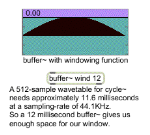
Making the decision between using a ‘buffer~’ or ‘jit.matrix’ to store the DSTFT data was one that I considered intensively. Up until last week it has been slightly unclear as to how this choice will affect me further down the line in the project. While I’ve been trying to come to a decision, I’ve also been considering whether using the objects in tandem could be a possibility to ensure I get maximum functionality out of both. In terms of storage of data, the answer to that is essentially no, the choice is whether to store data in one form or the other: you can store it in both if you like but wouldn’t be for the betterment of the project. Having chosen to collect DSTFT data through the ‘fftin~’ object and store it in a ‘jit.matrix’, there is one way in which buffer~ can be used alongside my patch. With ‘buffer~’ you can store a custom windowing function that can be called by the ‘fftin~’ object, but this is not a useful function for me as I have chosen to use the hanning window (which is already incorporated into the ‘fftin~’ object as it provides no amplitude modulation and a clean envelope.
Cycling 74’s article has also cleared up how ‘jit.poke~’ is synchronised with the data output from the DSTFT and then used to place this data in a ‘jit.matrix’. Specifically it was learning about how the 2nd inlet in this object controls the horizontal data placement and how the 3rd controls the vertical placement that that helped me grasp how ‘jit.poke~’ works in the DSTFT data collection process.
Had a meeting with my supervisor to discuss using ‘jit.gl.slab’ as an alternative to non-slab jitter processes. The reason behind this discussion was that in both Jean François-Charles’ and Tadej Droljc’s projects they mentioned the processes they outlined (in regular CPU-based jitter operators) are all possible in GPU-based slab processes. They continue to explain that processing as much of the project in the GPU will increase the speed of the project as a whole, yet neither explore GPU-based slab processes in much detail.
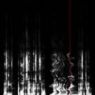
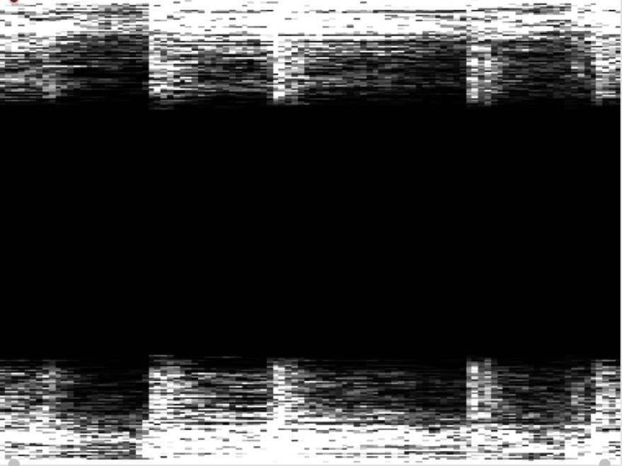
It is worth learning to walk before I can run though: CPU vs. GPU implementations will be something that becomes important when applying spectral processes, for now I have ensured that displaying the data in a traditional linear and logarithmically scaled spectrogram is the priority. When I first displayed DSTFT data in a ‘jit.pwindow’ it looked like this:
DSTFT linear spectrogram as of mid-January 2019
Clearly something wasn’t right, and I realised the issue was that I was packing the frame size with the number of frames and setting those as the dimensions of the jit.matrix, rather than packing the spectral frame size with the number of frames. Why this differentiation is important is explained in section ‘1.1 main’ of the project writeup, but essentially what is happening there is the DSTFT data is being mirrored about 0.5Sr (half the sample rate a.k.a the Nyquist frequency)
Week 3
Now that my linear spectrogram is functional, I am beginning to think about different ways in which I can visually render the DSTFT data. The world of Jitter seems almost like learning a new language in and of itself, and to attempt to navigate this I am currently looking through books 1, 2 and 3 of Andrew Bensons’s Jitters recipes. The books are somewhat seminal in the Max community and touch on a lot of functionality Jitter can offer.
For readers interesting in spectral data rendering or rendering of any large data set I would recommend these ‘recipes’ in particular:
Of the Jitter objects featured in these recipes, I am particularly interested in:
jit.coerce (change one matrix data type to another) jit.repos (manipulate one matrix using another as a spatial map) jit.gl.nurbs (renders a NURBS surface of any shape onto which we can map matrices (e.g. from a jit.gl.slab)) jit.dinmap (remap/ invert matrix dimensions) jit.rota (quick 2D scaling and rotation of matrices) jit.gl.isosurf (GL based surface extraction – investigate further) jit.gl.mesh (create a geometric surface from a jit.matrix)
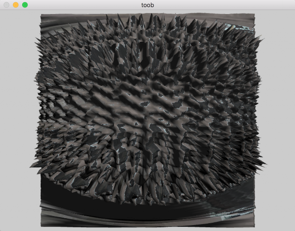
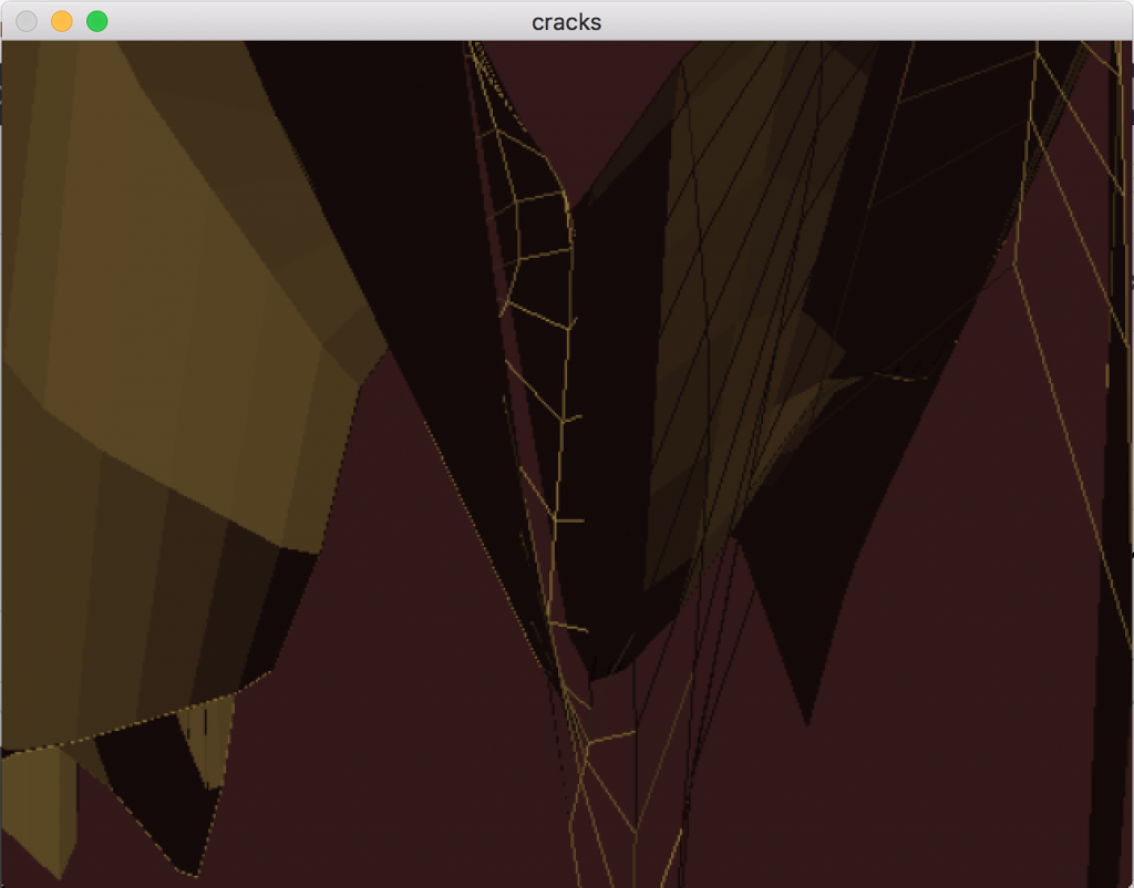
As I explore the capabilities for visualisation through jitter in my project further, a clear fork in the road is appearing ahead: do I opt for a large variety of malleability of rendering matrices in 3 dimensions (à la Andrew Bensons Jitter Recipes) at the sacrifice of control over the data, or the more simplistic two dimensional spectral processes with more possibility for user interaction that are outlined by Jean François-Charles and Tadej Droljc.
Week 4
The more I have considered what kind of project I want this to be, the more I realise that presenting a functional tool for the community is what I want to do.
Rendering the data in a form similar to the two above images would lend itself to a project that was more performance based, rather than being a more functional tool like I want my project to be. For sake of comparison here are the more functional linear and logarithmic spectrogram rendering contexts that I decided to use in my project:
Linear spectrogram Logarithmic spectrogram
Week 6
I am starting to struggle with patch latency issues and investigating processing data in the GPU via ‘jit.gl.slab’.
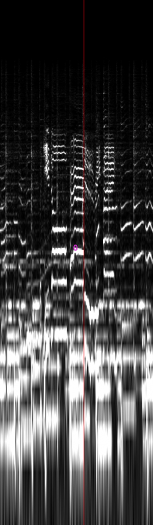
Investigating using Max’s shader .jxf files for ‘jit.gl.slab’. I am considering using an rendered external window to display spectrogram as there is less lag and exploring a way to be able to click on specific points of it and receive information about the click point. Scaling the spectrogram logarithmically in the SLAB version of ‘jit.repos’ sets a new spectrogram at each point of the logarithm rather than scaling one spectrogram throughout the whole window. The logarithmic spectrogram processed through ‘jit.gl.slab’ as of the 23rd February (and displayed through openGL ‘jit.window’) is in the image below.
Incorrectly scaled logarithmic spectrogram rendered through ‘jit.gl.slab’
Shader .jxf files directory: /Users/jack/Library/Mobile Documents/com~apple~CloudDocs/Documents/Max 8/Older version examples/examples (5.1.9)/jitter-examples/render
Week 7
Both spectrograms are now being rendered in external ‘jit.windows’. Inside both of their respective mapping abstractions and the global ‘circleclickpoint_&_line_alphablend’ abstraction I have replaced mapping abstraction dimension inverting, colour inverting and the alphablend with openGL equivalents. I have also replaced all instances of the jit.matrix with ‘jit.gl.slab’ where I can.
Objectives for the week:
1. Figure out a user-friendly way to interact with the spectrograms for time, amplitude and frequency information. 2. Find out how to close one spectrogram when using the other (this will speed up the project as a whole!). 3. Begin to integrate more spectral manipulation effects in as much openGL as possible. 4. Implement feature where all the DSTFT data is read into the matrix in one operation.
I realised that part of the reason why the patch was performing so slowly (mentioned in the semester 2 week 6 post on the 25/2/19) was because I had certain parts of the ‘jit.window’ rendering process (‘jit.window’ render rate, and line segment refresh rate in the alphablend) updating unnecessarily quickly – I have slowed them all down and the patch is running smoothly again.
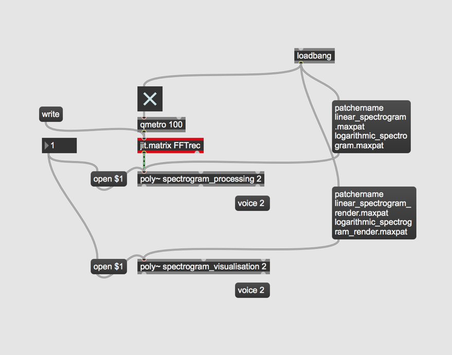
Going to investigate using ‘poly~’ to encapsulate each spectral processing routine with the resultant processed matrix still being displayed in a ‘jit.pwindow’. ‘poly~’ is proving to be very problematic for processing openGL: rendering contexts are not being established when the ‘poly~’ is opened. ‘horizontal_sync~’ is also having trouble being sent inside the ‘poly~’, meaning that the red line playback point in each spectrogram is not syncing correctly with the audio.
Week 8
Going to abandon use of ‘poly~’: instead I will save the matrix contents in the ‘pfft~’ in ‘1.1 main’ as .jxf files, then set the project to load this file into each spectral effect when it is opened by the user.
The abandoned poly~ idea
In the interest of CPU power, I have set the max sample size to be 1000 frames in the ‘stft_matrix_fill’ patch. Once play through has completed the matrix contents are saved as a .jit.jxf binary file whose name is the name of the loaded sample. I intend to continue expanding the project in this way, whereby the user will first record a chosen sample as a .jxf file, manually open whatever audio manipulation patch they want, where the .jxf file is loaded, and be able to use the patch henceforth. This limits the real-time aspect of the project, but since the spectral processing routines I intend to build are not designed for live input this doesn’t particularly matter.
I used Jean François Charles’ explanation of stochastic spectral synthesis for a ‘simpleplayback’ sub-patch that I have attached to the patches from 1.2.1 – 1.2.2 and 1.4.1 – 1.6.3. I have now also incorporated playback through stochastic synthesis, frame interpolation and transient based playback. I have made these 4 playback techniques abstractions so that the user will have the choice of 4 playback options in every module of the project. After learning that it is possible to monitor mouse position in the ‘jit.window,’ I have created an abstraction that first learns the user’s display resolution, and then adjusts the vertical dimensions of the ‘jit.window’ accordingly. Due to the scaling that occurs in ‘jit.window_dimensions’, the oval clickpoint doesn’t line up with the cursor at the perimeter of the ‘jit.window’. I fixed this by adjusting the scaling factors on ‘jit.gl.videoplane’ to 0.82 0.84 0.82.